【Python株価分析:第2回】株価データの可視化(Matplotlib & Plotly編)
前回はPythonを使ってYahoo!ファイナンスなどから株価データを取得する方法を解説しました。
今回はその取得した株価データを可視化して、「どのように価格が動いているか」「どのタイミングで投資判断をすべきか」などを視覚的に把握できるようにしていきます。
目次
本記事の目的
- 株価データを 折れ線グラフ で表示する
- 出来高や移動平均線(SMA)を表示して、相場の流れを把握
- インタラクティブなグラフで複数銘柄の比較を行う
※20日移動平均線とは、過去20日間の価格(通常は終値)の平均値を結んで描かれた線です。株価や為替レートなどの価格変動のトレンドを把握する際に利用されるテクニカル指標の一つです
使用ライブラリ
pip install pandas yfinance matplotlib plotlypandas: データ操作
yfinance: 株価データ取得
matplotlib: 静的な可視化
サンプルコード①:Matplotlibでシンプルに可視化
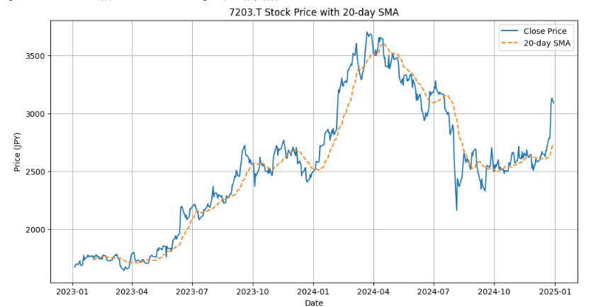
ポイント
rolling().mean()で簡単に移動平均を算出- プロットを重ねることで、売買判断の視覚化が可能に!
import yfinance as yf
import pandas as pd
import matplotlib.pyplot as plt

# 株価データを取得
ticker = "7203.T"  # トヨタ自動車
df = yf.download(ticker, start="2023-01-01", end="2024-12-31")

# 移動平均線(20日)
df["SMA_20"] = df["Close"].rolling(window=20).mean()

# プロット
plt.figure(figsize=(12,6))
plt.plot(df["Close"], label="Close Price")
plt.plot(df["SMA_20"], label="20-day SMA", linestyle='--')
plt.title(f"{ticker} Stock Price with 20-day SMA")
plt.xlabel("Date")
plt.ylabel("Price (JPY)")
plt.legend()
plt.grid(True)
plt.show()
サンプルコード②:Plotlyでインタラクティブ可視化
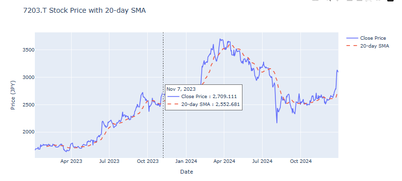
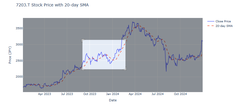
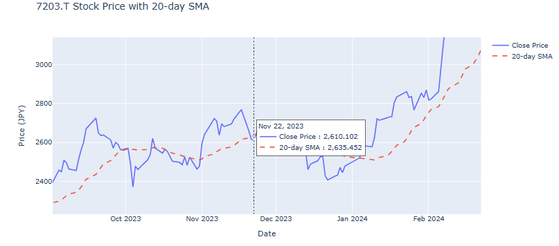
📌 ポイント
- マウスオーバーで詳細を確認できる
- ズームやパン操作で長期間の比較が可能
import yfinance as yf
import pandas as pd
import plotly.graph_objects as go
# 株価データの取得(日本株: トヨタ)
ticker = "7203.T"
df = yf.download(ticker, start="2023-01-01", end="2024-12-31", group_by='ticker')
# カラム名の整備(df["Close"] でアクセスできるように)
if isinstance(df.columns, pd.MultiIndex):
df.columns = df.columns.droplevel(0) # 1階層だけにする
# 移動平均線(20日)
df["SMA_20"] = df["Close"].rolling(window=20).mean()
# プロット
fig = go.Figure()
fig.add_trace(go.Scatter(x=df.index, y=df["Close"], mode="lines", name="Close Price"))
fig.add_trace(go.Scatter(x=df.index, y=df["SMA_20"], mode="lines", name="20-day SMA", line=dict(dash="dash")))
fig.update_layout(
title=f"{ticker} Stock Price with 20-day SMA",
xaxis_title="Date",
yaxis_title="Price (JPY)",
hovermode="x unified",
width=1000,
height=500
)
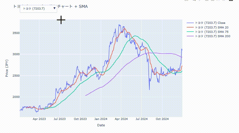
fig.show()複数銘柄をSMAと一緒にプロット
複数の日本株銘柄の株価をインタラクティブに切り替えながら可視化するグラフを作成しました。このチャートでは、各銘柄の終値(Close)に加え、20日・75日・200日の移動平均線(SMA)も一緒に表示できます。
さらに、ドロップダウンメニューから個別銘柄を選択できるほか、「すべての銘柄を表示」ボタンで全銘柄を重ねて比較することも可能です。
import yfinance as yf
import pandas as pd
import plotly.graph_objects as go

# 銘柄リスト
tickers = {
    "トヨタ (7203.T)": "7203.T",
    "ソニー (6758.T)": "6758.T",
    "キーエンス (6861.T)": "6861.T"
}

# データ取得と整形
data_dict = {}
for name, ticker in tickers.items():
    df = yf.download(ticker, start="2023-01-01", end="2024-12-31", group_by="ticker")
    if isinstance(df.columns, pd.MultiIndex):
        df.columns = df.columns.droplevel(0)

    if df.empty or "Close" not in df.columns:
        print(f"{ticker} のデータが取得できませんでした。スキップします。")
        continue

    df["SMA_20"] = df["Close"].rolling(window=20).mean()
    df["SMA_75"] = df["Close"].rolling(window=75).mean()
    df["SMA_200"] = df["Close"].rolling(window=200).mean()
    data_dict[name] = df

# グラフ作成
fig = go.Figure()
buttons = []
trace_names = []

# 各銘柄 + SMA をトレースとして追加
for i, (name, df) in enumerate(data_dict.items()):
    fig.add_trace(go.Scatter(x=df.index, y=df["Close"], mode="lines", name=f"{name} Close", visible=(i == 0)))
    fig.add_trace(go.Scatter(x=df.index, y=df["SMA_20"], mode="lines", name=f"{name} SMA 20", visible=(i == 0)))
    fig.add_trace(go.Scatter(x=df.index, y=df["SMA_75"], mode="lines", name=f"{name} SMA 75", visible=(i == 0)))
    fig.add_trace(go.Scatter(x=df.index, y=df["SMA_200"], mode="lines", name=f"{name} SMA 200", visible=(i == 0)))
    trace_names.append(f"{name} Close")

# ドロップダウンボタン作成
for i, name in enumerate(data_dict.keys()):
    visible = [False] * (len(data_dict) * 4)
    for j in range(4):
        visible[i * 4 + j] = True
    buttons.append(dict(
        label=name,
        method="update",
        args=[{"visible": visible},
              {"title": f"{name} の株価チャート + SMA"}]
    ))

# 「すべて表示」ボタン
buttons.append(dict(
    label="すべて表示",
    method="update",
    args=[{"visible": [True] * (len(data_dict) * 4)},
          {"title": "すべての銘柄を表示"}]
))

# レイアウト
fig.update_layout(
    title=f"{list(data_dict.keys())[0]} の株価チャート + SMA",
    xaxis_title="Date",
    yaxis_title="Price (JPY)",
    hovermode="x unified",
    updatemenus=[dict(
        active=0,
        buttons=buttons,
        direction="down",
        x=0,
        xanchor="left",
        y=1.15,
        yanchor="top"
    )],
    width=1000,
    height=600
)

fig.show()
応用編:出来高と価格を一緒にプロット
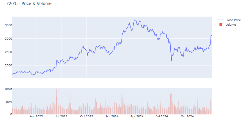
fig = make_subplots(rows=2, cols=1, shared_xaxes=True, vertical_spacing=0.1,
                    row_heights=[0.7, 0.3])

fig.add_trace(go.Scatter(x=df.index, y=df["Close"], name="Close Price"), row=1, col=1)
fig.add_trace(go.Bar(x=df.index, y=df["Volume"], name="Volume"), row=2, col=1)

fig.update_layout(title=f"{ticker} Price & Volume", height=600)
fig.show()
🧭 まとめ
| 内容 | ツール | ポイント |
|---|---|---|
| シンプル可視化 | Matplotlib | 移動平均やトレンドの確認に便利 |
| インタラクティブ可視化 | Plotly | 詳細な操作・分析に便利 |
| 出来高の分析 | Plotly + Bar | 市場の盛り上がりを視覚化 |
続きはこちら